AWS buys DuckLabs and about DuckDB with NetApp storage
- (this post): AWS buys DuckLabs and about DuckDB with NetApp storage
- follow up post: DuckDB Quack server with NetApp Storage
Introduction
DuckLabs are getting acquired by AWS.
The press release says:
Together, we'll make AWS analytics faster, simpler, and more cost-effective for customers.
Why DuckDB
I've been using DuckDB for a while, and even in the recent blog posts.
DuckDB works well with S3, it's very fast and provides a superior developer and operations experience.
What "faster, simpler, and more cost-effective" means is less Spark, more DuckDB.
People have been wondering about this for years. Not whether DuckDB can "replace Spark" (it still can't), but whether a lot of Spark cluster instances (on the low-end) are unnecessary because DuckDB can do the task faster, simpler, and more cost-effective.
I just tried this TPC-H variant with SF=20, to have an example (see Appendix A).
I ran it on a server with old CPUs, so it was not as fast as it would be if on modern hardware used for analytics today, but the point is you can max out 32 CPUs and get a lot of work done by a single DuckDB instance. It didn't even use much RAM, so it's a nice showcase for:
- Very short startup time
- Good compute scaling
- Fast and efficient performance
- Runs serverless (in-process)
For smaller jobs (load 100-200 MB CSV to data lake), DuckDB can finish before Spark is done starting up.
In other cases (large jobs where CPU or RAM of one system isn't enough) DuckDB will run much slower, but if it takes 3 minutes to complete vs 1 minute on a Spark cluster, you spend 90% less and still finish within 5 minutes.
You can do your own warehouse loading or other tests that match your low-end Spark workload, and realize you don't need to run Spark clusters for those.
DuckDB with NetApp storage
StorageGRID first, because it's where most DuckDB users should store databases or where they'll access data lake tables. Simply use httpfs (see here) to get started. If you have Delta or Iceberg tables, there are plugins for those, too (both read and write, although one has to attach to a catalog to be able to write).
E-Series is great for local DuckDB tables if you need to keep data files on protected storage: you can get excellent random and sequential performance even from an entry level EF-Series model which can concurrently serve dozens of DuckDB clients. If you need to automate storage provisioning, you can do it with Ansible or Terraform or leave it to a CSI driver such as TopoLVM.
Tables or files can also be created locally and uploaded to S3. For smaller applications, it is sometimes possible to download from S3 and upload on shutdown.
TFM says this about large DuckDB databases:
- DuckDB's native database format supports huge database files without any practical restrictions
- Object storage systems have lower limits on file sizes than block-based storage systems. For example, AWS S3 limits the file size to 5 TB.
- Checkpointing a DuckDB database can be slow. For example, checkpointing after adding a few rows to a table in the TPC-H SF1000 database takes approximately 5 seconds.
- On block-based storage, the file system has a significant effect on performance when working with large files. On Linux, DuckDB performs best with XFS on large files.
Most of these won't bother you with small and mid-sized DBs, and remember that you don't have to use the native database format. Datalakes don't put everything in one file - and you can partition tables in DuckDB before upload - so you won't have that S3 problem.
For native DuckDB, XFS on E-Series will work well. Here you can see a multi-threaded workload that gets multiple GB/s from a single protected disk (LUN). You won't save much using storage that compresses data because it's done by the client (DuckDB, that is), but E-Series doesn't have compression so you only gain from built-in compression.
Let's take a look at the documents table from my post on agentic RAG where local.duckdb was used to store documents, chunks, and embeddings:
local D SELECT * EXCLUDE (column_path, segment_id, start, stats, persistent, block_id, block_offset)
      FROM pragma_storage_info('docs') USING SAMPLE 10 ROWS ORDER BY row_group_id;
┌──────────────┬─────────────┬───────────┬───┬─────────────┬─────────────┬──────────────┬──────────────────────┐
│ row_group_id │ column_name │ column_id │ … │ compression │ has_updates │ segment_info │ additional_block_ids │
│    int64     │   varchar   │   int64   │ … │   varchar   │   boolean   │   varchar    │       int64[]        │
├──────────────┼─────────────┼───────────┼───┼─────────────┼─────────────┼──────────────┼──────────────────────┤
│            0 │ embedding   │         3 │ … │ ALPRD       │ false       │              │ []                   │
│            0 │ embedding   │         3 │ … │ ALPRD       │ false       │              │ []                   │
│            1 │ embedding   │         3 │ … │ Constant    │ false       │              │ []                   │
│            1 │ title       │         1 │ … │ Constant    │ false       │              │ []                   │
│            2 │ embedding   │         3 │ … │ ALPRD       │ false       │              │ []                   │
│            2 │ embedding   │         3 │ … │ Constant    │ false       │              │ []                   │
│            2 │ title       │         1 │ … │ Dictionary  │ false       │              │ []                   │
│            3 │ doc_id      │         0 │ … │ Constant    │ false       │              │ []                   │
│            3 │ embedding   │         3 │ … │ Constant    │ false       │              │ []                   │
│            3 │ chunk_index │         4 │ … │ Constant    │ false       │              │ []                   │
└──────────────┴─────────────┴───────────┴───┴─────────────┴─────────────┴──────────────┴──────────────────────┘
  10 rows                         use .last to show entire result                          9 columns (7 shown)
All columns are compressed and I didn't have to do anything (in fact, I expected some may be compressed, but didn't look until now).
Here's what two of them mean (no idea what ALPRD is) from the post above:
- Constant encoding is the most straightforward compression algorithm in DuckDB. Constant encoding is used when every single value in a column segment is the same value
- Dictionary encoding works by extracting common values into a separate dictionary, and then replacing the original values with references to said dictionary
And finally, E-Series is also good for larger-than-RAM workloads if your local disk space is limited because spillover-to-disk can use E-Series. Simply create a RAID 10 or RAID 0 disk group and a LUN for each DuckDB client. If you have 16 servers that run DuckDB workloads and each needs 1TiB of disk cache, take several disks, create a disk group with 16TiB usable capacity, create 16 volumes and assign them to your DuckDB servers. Each server mounts its scratch disk to /tmp/duckdb and then: SET temp_directory = '/tmp/duckdb';. Have 4 servers per disk for fast performance, although you can have more if overflows to disk aren't concurrent.
For remote access - including in hybrid cloud - simply use StorageGRID because you don't have to deal with storage presentation and management: you get unlimited capacity and end-to-end HTTPS encryption, which beats unencrypted iSCSI and NFS.
There's a simple COSI driver to automate that and bucket snapshots, too, so that you can get to a Point-in-Time DuckDB and run read-only reports based on it. The recommended way is to use a datalake, though, so that you don't have to use these "storage tricks".
Backup and restore
Use the correct way unless DB grows to an unmanageable size:
memory D ATTACH '/mnt/dm-7/duckdb/duckdb-tpch-power-test/gen/sf100/tpch_template.duckdb' AS db (READ_ONLY);
memory D ATTACH './backup.duckdb' AS backup;
memory D COPY FROM DATABASE db TO backup;
With both DBs on one RAID 6 (10 disks, 8 data, 2 parity) of E-Series E4000, I get 470 MB/s. It took me some 60 seconds to backup this DB to the same disk:
-rw-r--r-- 1 sean sean 27G Sep 14 10:53 backup.duckdb
It'd take 36 minutes to backup a TB-sized DuckDB this way.
I know this RAID 6 disk group can deliver well over 1 GB/s, so the bottleneck isn't on storage.
If that doesn't work for you (database is "too large"), use storage-side snapshots:
- E-Series has them - do it manually or automate (see an example). In Kubernetes, I can do that with IBM Block CSI with SANtricity patches. SANtricity CSI not yet, because I'm not a big believer in array snapshots for modern workloads. (If you read this post carefully you'll see restores aren't done from the snapshot - although you could do it directly on array, but from a backup copy - the way it's supposed to be done in Kubernetes.)
- StorageGRID can take them, too. Do it manually (see bucket snapshots) or automate. Oh, I can automate that in Kubernetes, too, using COSI snapshots. You'd also have to create and claim a snapshot (bucket), then copy database or its selected objects from the snapshot bucket to your "production" bucket.
Conclusion
DuckDB is already reasonably well-known, but probably not fully mainstream - especially not in the enterprise. AWS is going to change that.
It's always nice to see JVM bloatware removed from places where it adds no value. I'm sure AWS will make good use of DuckDB, and - related to my expectations from S3-focused posts - DuckDB is going to play a much larger role going forward with S3 as its main target.
If you have workloads that look even remotely suitable for DuckDB - not just Spark, but any workload and format supported by DuckDB - I strongly recommend evaluating DuckDB - especially if you already have StorageGRID.
Appendix A: Results with Scale Factor 20
It's not something to compare against, but to give an idea - the details of the CPU-maxing run done above.
- Ubuntu 26.04 LTS
- DuckDB v1.5.5
- Old Xeon Silver CPU external disk (NVMe/RoCE; NeApp EF-Series EF600)
- Intel(R) Xeon(R) Silver 4110 CPU @ 2.10GHz
- 32 vCPU (2 x 8 cores, HT enabled)
- duckdb-tpch-power-test, SF=20 (as of August 31, 2026)
tpch_load_time                  = 62.6 seconds
throughput_measurement_interval = 21.53
power_total_queries_duration    = 9.42
tpch_power_at_size              = 251009.67
tpch_throughput_at_size         = 220715.28
tpch_qphh_at_size               = 235375.59
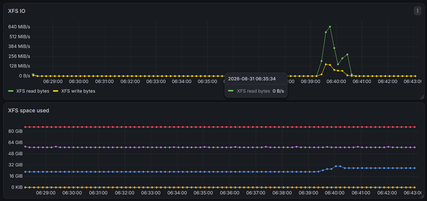
It is obvious from the screenshot above (and the Grafana screenshot below) that CPU was the bottleneck and storage wasn't that busy, which tells me dozens of such workloads could run against a single EF-Series array as long as CPUs and RAM were enough.
Log:
time_offset	cpu_percent	cpu_user	cpu_system	memory_rss	memory_vms	read_bytes	write_bytes
0.01	0	851.52	41.83	158060544	5906333696	0	0
1.02	1360	861.29	45.69	1830797312	6065762304	1242771456	6316032
2.02	2518	883.71	48.53	2537811968	6334197760	2350907392	6356992
3.03	2613	907.36	51.13	4185939968	6602633216	2788548608	6356992
4.04	2729	933.21	52.7	4219371520	6602633216	3419426816	6373376
5.04	2735	960.05	53.53	4401254400	7072399360	3583111168	6373376
6.05	2919	987.43	55.6	4972711936	7407939584	3947290624	6545408
7.05	2265	1008.85	56.83	5149765632	7407939584	4151943168	6545408
8.06	2843	1034.18	60.1	6307704832	8414580736	4157186048	6545408
9.06	2706	1061.31	60.29	5511450624	7609266176	4157186048	6553600
10.07	2704	1088.03	60.64	5563731968	7844229120	4173553664	7770112
11.08	3139	1118.97	61.25	5800771584	7978455040	4173553664	14475264
12.08	3055	1149.16	61.9	6009622528	8246878208	4173553664	20525056
13.09	3174	1180.48	62.46	5896044544	8112648192	4173553664	20525056
14.1	3181	1211.27	63.66	6440906752	8649523200	4173553664	20525056
15.1	3174	1240.53	66.41	7434584064	9723269120	4173553664	20525056
16.11	3148	1271.26	67.39	8239038464	10729902080	4173553664	21180416
17.12	3050	1301.47	67.89	7215255552	8917958656	4173553664	21180416
18.12	3038	1331.92	68.03	7143301120	8783740928	4173553664	21286912
19.13	3086	1361.25	69.82	8063709184	9857486848	4173553664	23138304
20.14	3147	1392.79	70.02	7767265280	10461466624	4173553664	23138304
21.15	3108	1423.5	70.43	7415472128	9119289344	4173553664	23244800
22.16	3169	1455.16	70.72	7423406080	9186398208	4174667776	23244800
23.16	3180	1487.13	70.9	7436144640	9219952640	4174667776	23244800
24.17	3184	1518.56	71.49	7491637248	9521934336	4174667776	23433216
25.18	3136	1549.71	71.98	7483817984	9219948544	4174667776	23433216
26.19	3015	1579.52	72.45	7499300864	9253502976	4174667776	23498752
27.2	3075	1610.19	72.91	7600840704	9253511168	4174667776	23498752
28.2	3058	1640.24	73.66	7517065216	9253502976	4174667776	23498752
29.21	3048	1668.98	75.7	8357429248	10193035264	4174667776	23498752
30.22	3149	1700.22	76.17	7485153280	9320607744	4174667776	23506944
31.23	3079	1730.98	76.5	7572692992	9287061504	4174667776	23572480
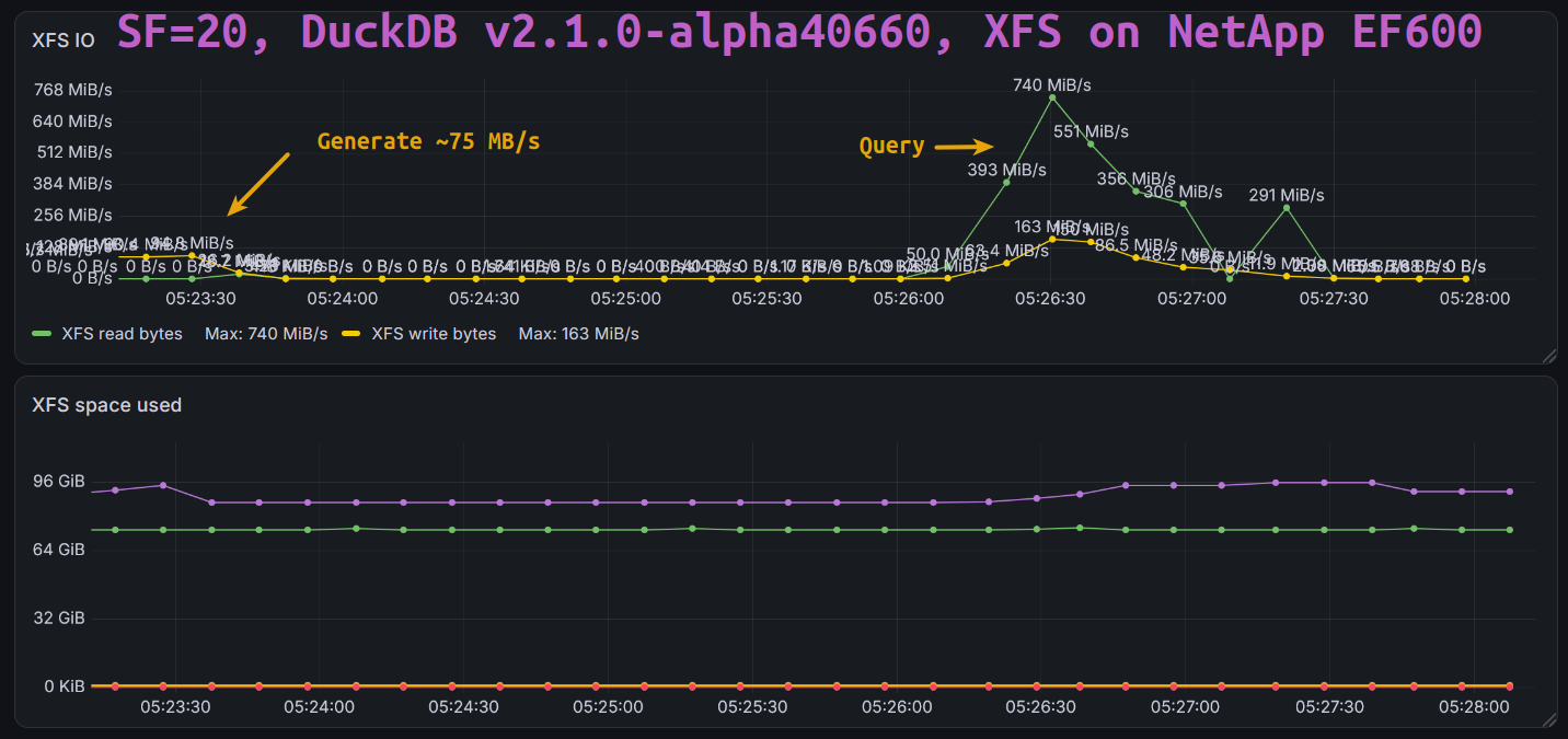
This is the same view from Grafana shows moderate activity on the array (not even 1 GB/s).
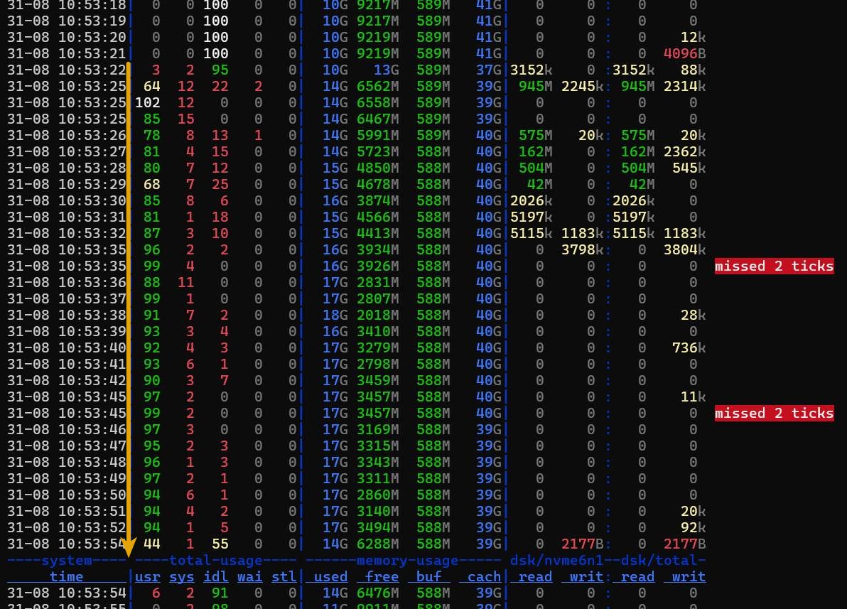
I wanted to capture RAM utilization, so I executed another run on existing data.
tpch_load_time                  = n/a (ran on cached database)
throughput_measurement_interval = 21.26
power_total_queries_duration    = 9.50
tpch_power_at_size              = 236849.19
tpch_throughput_at_size         = 223518.34
tpch_qphh_at_size               = 230087.24
DuckDB didn't use a lot of RAM.
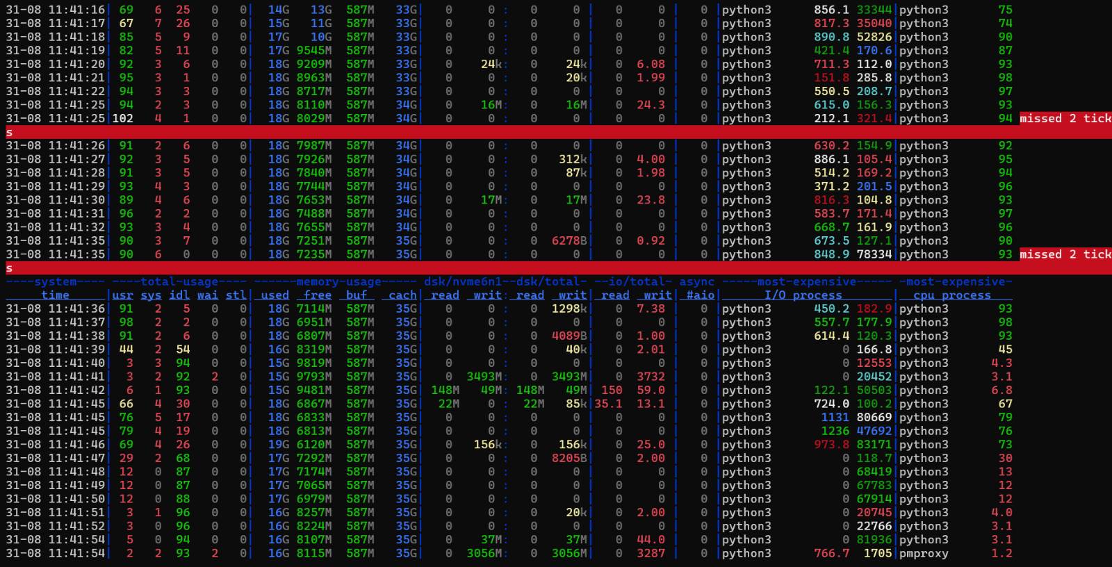
Another run (both load and query) was done to capture more details.
The result is similar, but we can see that the benchmark (python) writes can load data over 3 GB/s.
tpch_load_time                  = 60.2 seconds
throughput_measurement_interval = 21.79
power_total_queries_duration    = 8.78
tpch_power_at_size              = 262211.93
tpch_throughput_at_size         = 218081.69
tpch_qphh_at_size               = 239130.97
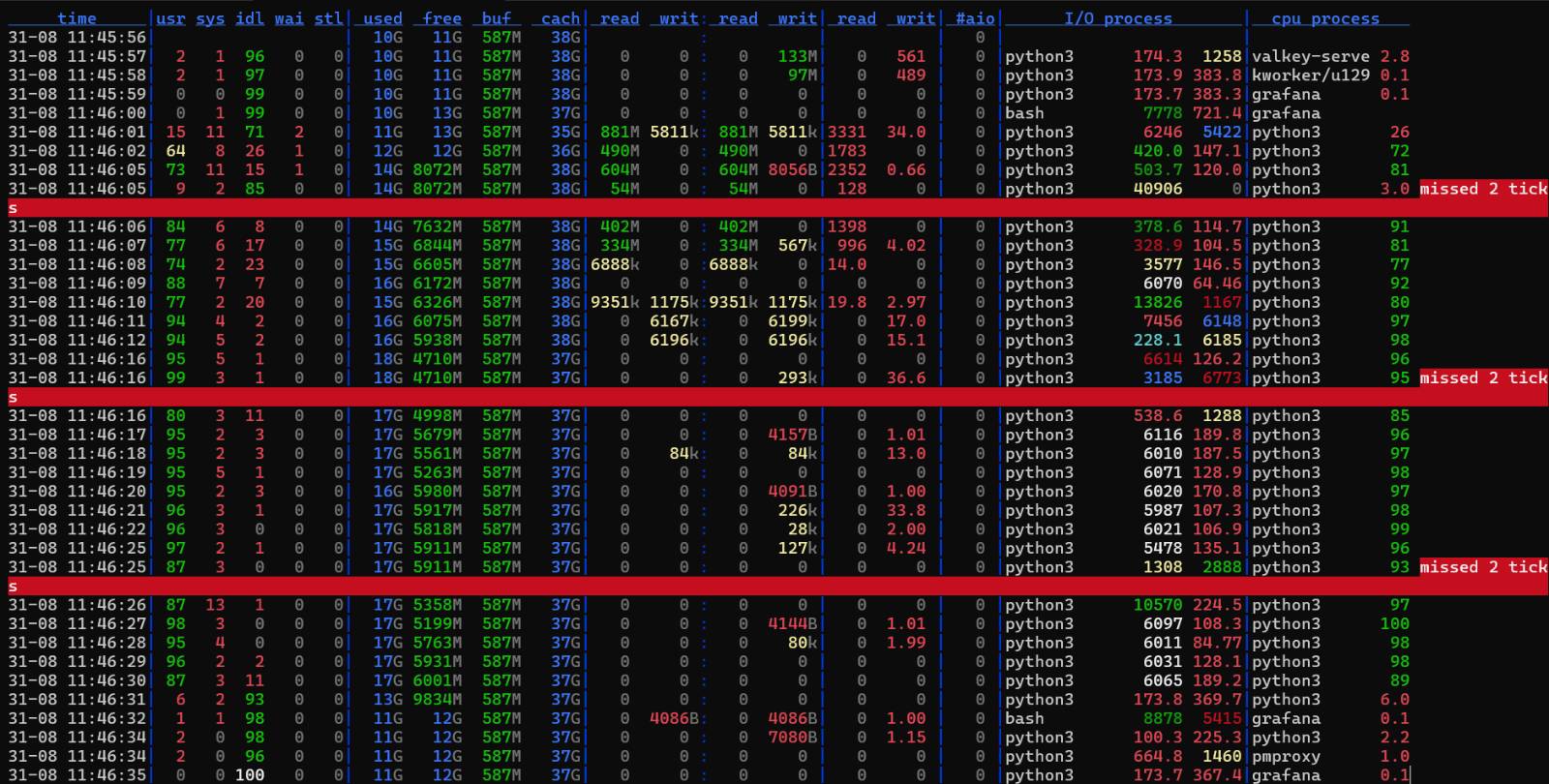
Another run (query only) shows consistent RAM utilization for queries across multiple runs.
Control write and read run with fio on the same volume using multi-threaded 1MiB read and write requests (async on write, directIO on read):
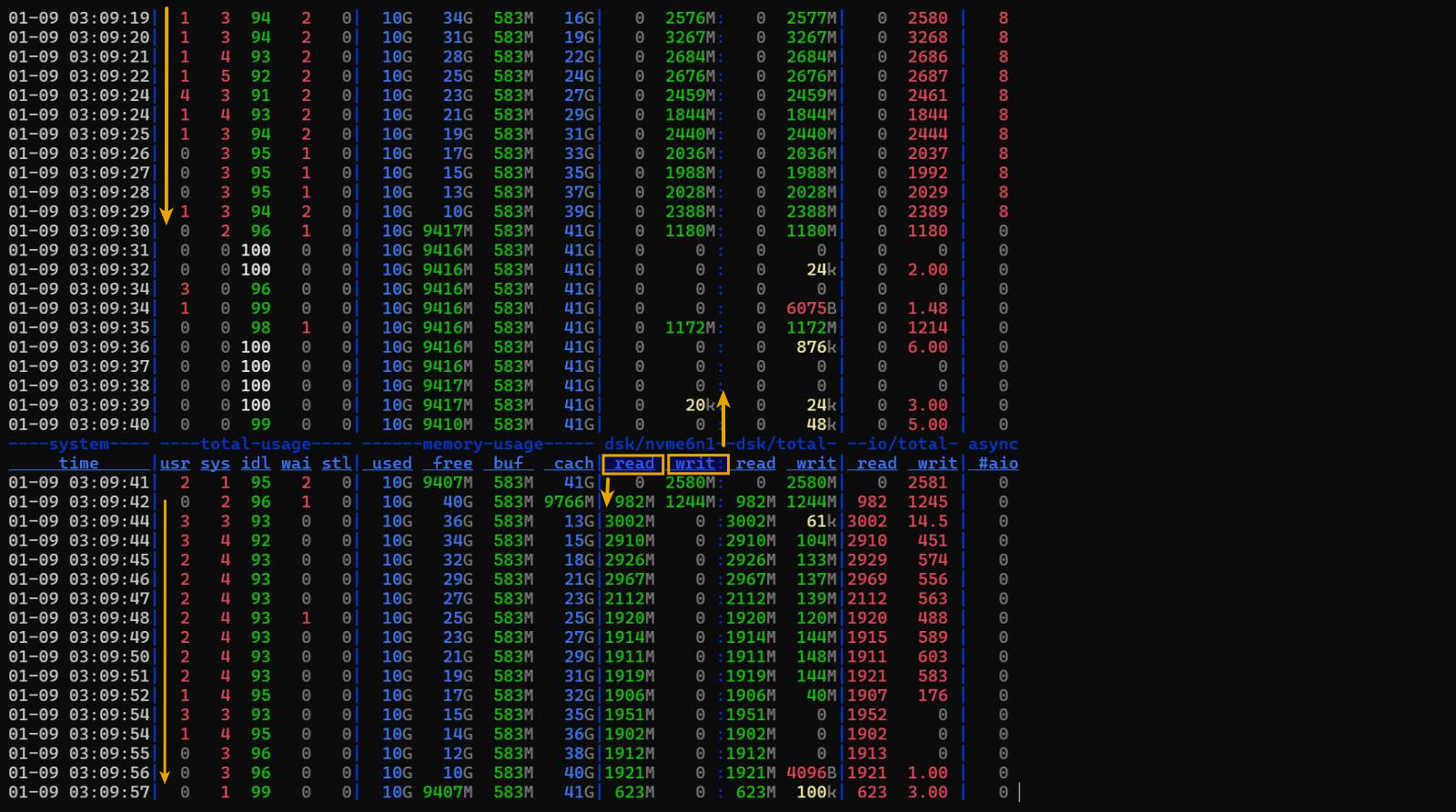
The read test was slower than normal due to queue depth 1 (set automatically by fio).
$ sudo fio --name=jobname --filename=/cache/testfile --size=32G --rw=write --bs=1M --numjobs=1 --thread=8 --iodepth=8 --ioengine=libaio
Tue Sep  1 03:11:37 AM UTC 2026
jobname: (g=0): rw=write, bs=(R) 1024KiB-1024KiB, (W) 1024KiB-1024KiB, (T) 1024KiB-1024KiB, ioengine=libaio, iodepth=8
fio-3.41
Starting 1 thread
Jobs: 1 (f=1): [W(1)][100.0%][w=2075MiB/s][w=2075 IOPS][eta 00m:00s]
jobname: (groupid=0, jobs=1): err= 0: pid=1860459: Tue Sep  1 03:11:52 2026
  write: IOPS=2333, BW=2334MiB/s (2447MB/s)(32.0GiB/14042msec); 0 zone resets
    slat (usec): min=303, max=1134, avg=420.53, stdev=63.05
    clat (usec): min=4, max=6016, avg=2969.91, stdev=431.79
     lat (usec): min=474, max=6855, avg=3390.44, stdev=492.55
    clat percentiles (usec):
     |  1.00th=[ 2311],  5.00th=[ 2442], 10.00th=[ 2474], 20.00th=[ 2507],
     | 30.00th=[ 2540], 40.00th=[ 2638], 50.00th=[ 3261], 60.00th=[ 3326],
     | 70.00th=[ 3326], 80.00th=[ 3392], 90.00th=[ 3425], 95.00th=[ 3458],
     | 99.00th=[ 3523], 99.50th=[ 3523], 99.90th=[ 4015], 99.95th=[ 5014],
     | 99.99th=[ 5866]
   bw (  MiB/s): min= 2042, max= 2884, per=100.00%, avg=2336.79, stdev=334.47, samples=28
   iops        : min= 2042, max= 2884, avg=2336.79, stdev=334.47, samples=28
  lat (usec)   : 10=0.01%, 500=0.01%, 1000=0.01%
  lat (msec)   : 2=0.01%, 4=99.88%, 10=0.10%
  cpu          : usr=11.07%, sys=88.85%, ctx=389, majf=0, minf=6181
  IO depths    : 1=0.1%, 2=0.1%, 4=0.1%, 8=100.0%, 16=0.0%, 32=0.0%, >=64=0.0%
     submit    : 0=0.0%, 4=100.0%, 8=0.0%, 16=0.0%, 32=0.0%, 64=0.0%, >=64=0.0%
     complete  : 0=0.0%, 4=100.0%, 8=0.1%, 16=0.0%, 32=0.0%, 64=0.0%, >=64=0.0%
     issued rwts: total=0,32768,0,0 short=0,0,0,0 dropped=0,0,0,0
     latency   : target=0, window=0, percentile=100.00%, depth=8

Run status group 0 (all jobs):
  WRITE: bw=2334MiB/s (2447MB/s), 2334MiB/s-2334MiB/s (2447MB/s-2447MB/s), io=32.0GiB (34.4GB), run=14042-14042msec

Disk stats (read/write):
  nvme6n1: ios=0/27689, sectors=0/56647704, merge=0/0, ticks=0/167340, in_queue=167340, util=51.94%

$ sudo fio --name=jobname --filename=/cache/testfile --size=32G --rw=read --bs=1M --numjobs=1 --thread=8 --iodepth=8
Tue Sep  1 03:09:40 AM UTC 2026
jobname: (g=0): rw=read, bs=(R) 1024KiB-1024KiB, (W) 1024KiB-1024KiB, (T) 1024KiB-1024KiB, ioengine=psync, iodepth=8
fio-3.41
Starting 1 thread
note: both iodepth >= 1 and synchronous I/O engine are selected, queue depth will be capped at 1
Jobs: 1 (f=1): [R(1)][100.0%][r=1921MiB/s][r=1921 IOPS][eta 00m:00s]
jobname: (groupid=0, jobs=1): err= 0: pid=1860330: Tue Sep  1 03:09:57 2026
  read: IOPS=2039, BW=2040MiB/s (2139MB/s)(32.0GiB/16065msec)
    clat (usec): min=120, max=6357, avg=446.46, stdev=765.10
     lat (usec): min=120, max=6357, avg=446.55, stdev=765.10
    clat percentiles (usec):
     |  1.00th=[  123],  5.00th=[  127], 10.00th=[  131], 20.00th=[  137],
     | 30.00th=[  147], 40.00th=[  172], 50.00th=[  180], 60.00th=[  186],
     | 70.00th=[  192], 80.00th=[  202], 90.00th=[ 1729], 95.00th=[ 2835],
     | 99.00th=[ 2933], 99.50th=[ 2966], 99.90th=[ 2999], 99.95th=[ 3032],
     | 99.99th=[ 3163]
   bw (  MiB/s): min=  480, max= 3042, per=100.00%, avg=2179.20, stdev=570.06, samples=30
   iops        : min=  480, max= 3042, avg=2179.20, stdev=570.06, samples=30
  lat (usec)   : 250=87.34%, 500=0.14%, 750=0.01%, 1000=0.01%
  lat (msec)   : 2=5.03%, 4=7.48%, 10=0.01%
  cpu          : usr=0.28%, sys=93.84%, ctx=509, majf=0, minf=1321
  IO depths    : 1=100.0%, 2=0.0%, 4=0.0%, 8=0.0%, 16=0.0%, 32=0.0%, >=64=0.0%
     submit    : 0=0.0%, 4=100.0%, 8=0.0%, 16=0.0%, 32=0.0%, 64=0.0%, >=64=0.0%
     complete  : 0=0.0%, 4=100.0%, 8=0.0%, 16=0.0%, 32=0.0%, 64=0.0%, >=64=0.0%
     issued rwts: total=32768,0,0,0 short=0,0,0,0 dropped=0,0,0,0
     latency   : target=0, window=0, percentile=100.00%, depth=8

Run status group 0 (all jobs):
   READ: bw=2040MiB/s (2139MB/s), 2040MiB/s-2040MiB/s (2139MB/s-2139MB/s), io=32.0GiB (34.4GB), run=16065-16065msec

Disk stats (read/write):
  nvme6n1: ios=32404/3861, sectors=66338816/7905280, merge=0/0, ticks=65654/38478, in_queue=104133, util=68.53%
Appendix B: DuckDB version 2
Differences compared to configuration in Appendix A are noted in list items.
- DuckDB v2.1.0-alpha40660 - upgraded from v1
Query only:
Logged to log-sf20-2026-09-08T05-16-41.765830+00-00.tsv

tpch_load_time                  = n/a (ran on cached database)
throughput_measurement_interval = 20.07
power_total_queries_duration    = 8.64
tpch_power_at_size              = 246200.99
tpch_throughput_at_size         = 236771.30
tpch_qphh_at_size               = 241440.11
- Add
read_ahead_depth=32andasync_threads=32
Full run:
Logged to log-sf20-2026-09-08T05-26-06.164243+00-00.tsv

tpch_load_time                  = 66.6 seconds
throughput_measurement_interval = 17.42
power_total_queries_duration    = 7.77
tpch_power_at_size              = 284180.39
tpch_throughput_at_size         = 272789.90
tpch_qphh_at_size               = 278426.90
All right, that is around 20% better than v1 even though the CPUs were a bottleneck even in v1.
As with v1, we can see the volume can deliver more - there is a hint of that at 05:27:14, but CPUs are the main bottleneck.
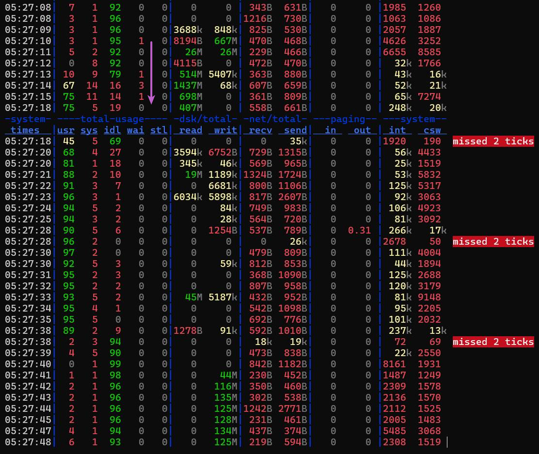
I didn't try higher values as CPUs were already maxed out.
Grafana samples were less frequent.
This final result is a TPC-H (SF100) run on a FC-connected E-Series E4012 with data on RAID 6 (NL-SAS, 8 disks, 2 parity), using DuckDB v2.0.0-alpha41533 (Cyanoptera) 10de957379.
Compared to NVMe with TCL, this was FC with NL-SAS, but it had 2 x AMD EPYC 9335 32-Core Processor.
tpch_load_time                  = 97.3 seconds
throughput_measurement_interval = 32.81
power_total_queries_duration    = 10.08
tpch_power_at_size              = 1155688.19
tpch_throughput_at_size         = 1206949.10
tpch_qphh_at_size               = 1181040.57